Show code cell source

Hide code cell source

import ase
import matplotlib.pyplot as plt
from ase.io import write

import abtem

4D-STEM quickstart

This notebook demonstrates a basic 4D-stem simulation of MoS₂.

Configuration

We start by (optionally) setting our configuration. See documentation for details.

abtem.config.set(
    {
        "device": "cpu",
        "fft": "fftw",
        "diagnostics.task_progress": True,
        "diagnostics.progress_bar": "tqdm",
    }
);

Atomic model

We create the atomic model. See our walkthough or our tutorial on atomic models.

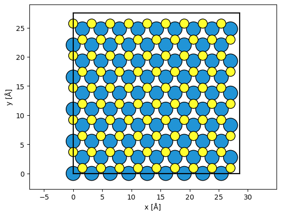
We create an atomic model of silicon using the mx2 function from ASE. The structure is repeated in order to improve the reciprocal space sampling of the simulation.

atoms = ase.build.mx2("WS2", vacuum=2)

atoms = abtem.orthogonalize_cell(atoms)

atoms = atoms * (9, 5, 1)

abtem.show_atoms(atoms)

(<Figure size 640x480 with 1 Axes>, <Axes: xlabel='x [Å]', ylabel='y [Å]'>)

Potential

We create an ensemble of potentials using the frozen phonon. See our walkthrough on frozen phonons.

frozen_phonons = abtem.FrozenPhonons(atoms, 8, sigmas=0.1)

We create a potential from the frozen phonons model, see walkthrough on potentials.

potential = abtem.Potential(frozen_phonons, sampling=0.05)

Wave function

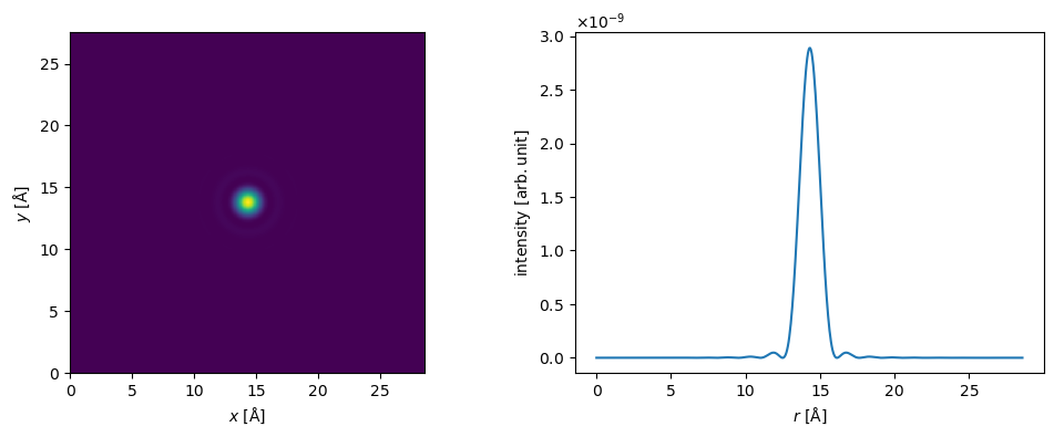
We create a probe wave function at an energy of \(80 \ \mathrm{keV}\), an objective aperture of \(12 \ \mathrm{mrad}\). See our walkthrough on wave functions.

Partial temporal coherence is neglected here, see our tutorial on partial coherence.

probe = abtem.Probe(energy=80e3, semiangle_cutoff=14)
probe.grid.match(potential)

fig, (ax1, ax2) = plt.subplots(1, 2, figsize=(12, 4))
probe.show(ax=ax1)
probe.profiles().show(ax=ax2);

Scan

We select a scan region using fractional coordinates. We scan at the Nyquist frequency, although there is no real reason to do that in a 4D-STEM simulation.

grid_scan = abtem.GridScan(
    start=[0, 0],
    end=[1 / 9, 1 / 5],
    fractional=True,
    potential=potential,
)

Detect

We use a flexible annular detector, this will let us choose the detector angles after the running multislice.

detector = abtem.PixelatedDetector(max_angle=200)

We set up the scanned multislice simulation. See our walkthrough on scanning and detecting.

measurements = probe.scan(potential, scan=grid_scan, detectors=detector)
measurements.array

Array Chunk Bytes 11.20 MiB 11.20 MiB Shape (5, 8, 277, 265) (5, 8, 277, 265) Dask graph 1 chunks in 39 graph layers Data type float32 numpy.ndarray

measurements.sampling

(0.034940600978336823, 0.03631133768488212)

We run the simulation directly to disk.

measurements.to_zarr("4d-stem_quickstart.zarr", compute=True);

The data is read back lazily. We load it into memory using .compute.

measurements = abtem.from_zarr("4d-stem_quickstart.zarr").compute()

Post-processing

We can simulate partial spatial coherence by applying a gaussian filter. The standard deviation of the filter is \(0.3 \ \mathrm{Å}\), the approximate size of the electron source.

filtered_measurements = measurements.gaussian_source_size(0.3)

Partial temporal coherence is neglected here, see our tutorial on partial coherence if you want to include this in your simulation.

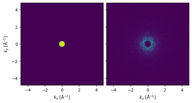
noisy_measurements = filtered_measurements.poisson_noise(dose_per_area=1e6)

We show one of the diffraction patterns below. To see the signal outside the bright field disk it may be necessary to block it.

abtem.stack((noisy_measurements[0, 0], noisy_measurements[0, 0].block_direct())).show(
    explode=True, title=None
)

<abtem.visualize.visualizations.Visualization at 0x1c698a990>

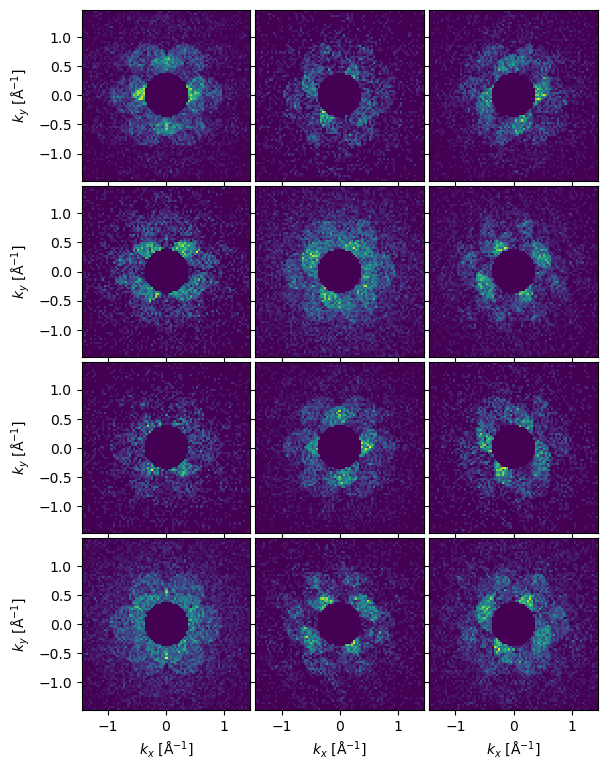
We can show the entire dataset as an exploded plot. If the dataset is large we can use numpy indexing to select every n’th diffraction pattern.

visualization = (
    noisy_measurements[::2, ::2]
    .crop(60)
    .block_direct()
    .show(explode=True, figsize=(8, 8), title=None)
)
visualization.axes.set_sizes(padding=0.05)

Reduction

abTEM features a few builtin methods for reducing 4D-stem dataset. For more sophisticated methods, see for example py4DSTEM or pyxem.

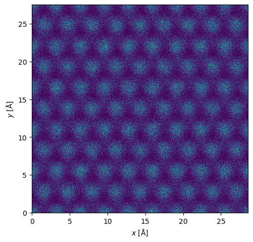
We can of course integrate the 4D-STEM dataset to get a ADF signal.

maadf = (
    filtered_measurements.integrate_radial(50, 150)
    .interpolate(0.05)
    .tile((9, 5))
    .poisson_noise(dose_per_area=1e5)
)

maadf.show();

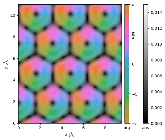
We can get the center of mass and integrated center of mass.

center_of_mass = filtered_measurements.center_of_mass()

interpolated_center_of_mass = center_of_mass.interpolate(0.05).tile((3, 2))

interpolated_center_of_mass.show(cbar=True, vmax=0.015, vmin=0);