Show code cell source

Hide code cell source

import ase
import matplotlib.pyplot as plt
import numpy as np
from ase.cluster import Decahedron

import abtem

PRISM quickstart

This is a short example of running a STEM simulation of a supported nanoparticle with the PRISM algorithm. See our tutorial for a more in depth description.

Configuration

We start by (optionally) setting our configuration. See documentation for details.

Atomic model

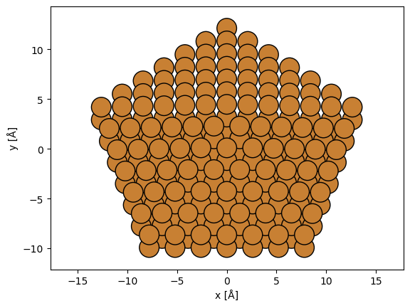
We create an atomic model of a decahedral copper nanoparticle. See our walkthough or our tutorial on atomic models.

cluster = Decahedron("Cu", 7, 2, 0)
cluster.rotate("x", 30)

abtem.show_atoms(cluster, plane="xy");

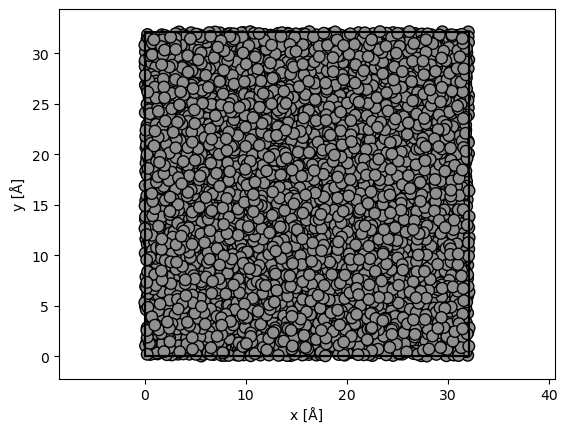
A rough model of amorphous carbon is created by randomly displacing the atoms of a diamond structure

substrate = ase.build.bulk("C", cubic=True)

# repeat diamond structure
substrate = substrate * (9, 9, 20)

# displace atoms with a standard deviation of 50 % of the bond length
bondlength = 1.54  # Bond length
substrate.positions[:] += np.random.randn(len(substrate), 3) * 0.5 * bondlength

# wrap the atoms displaced outside the cell back into the cell
substrate.wrap()

abtem.show_atoms(substrate, plane="xy", merge=0.5);

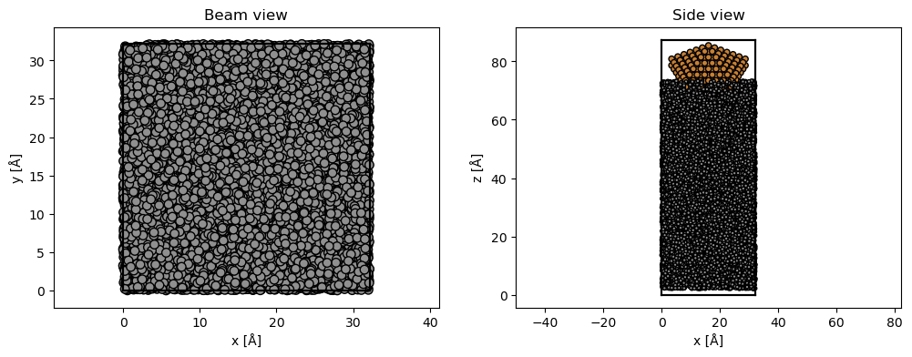
translated_cluster = cluster.copy()

translated_cluster.cell = substrate.cell
translated_cluster.center()
translated_cluster.translate((0, 0, 40))

atoms = substrate + translated_cluster

atoms.center(axis=2, vacuum=2)

fig, (ax1, ax2) = plt.subplots(1, 2, figsize=(12, 4))
abtem.show_atoms(atoms, plane="xy", ax=ax1, title="Beam view")
abtem.show_atoms(atoms, plane="xz", ax=ax2, title="Side view");

Potential

We create an ensemble of potentials using the frozen phonon model. See our walkthrough on frozen phonons.

frozen_phonons = abtem.FrozenPhonons(atoms, 8, sigmas=0.1)

We create a potential from the frozen phonons model, see walkthrough on potentials.

potential = abtem.Potential(
    frozen_phonons,
    gpts=512,
    slice_thickness=2,
)

SMatrix

We create the ensemble of SMatrices by providing our potential, an acceleration voltage \(200 \ \mathrm{keV}\), a cutoff of the plane wave expansion of the probe of \(20 \ \mathrm{mrad}\) and an interpolation factor of 4 in both \(x\) and \(y\). See our tutorial on PRISM for more details.

s_matrix = abtem.SMatrix(
    potential=potential,
    energy=100e3,
    semiangle_cutoff=20,
    interpolation=4,
    downsample=True,
)

s_matrix.shape

(8, 69, 512, 512)

Contrast transfer function

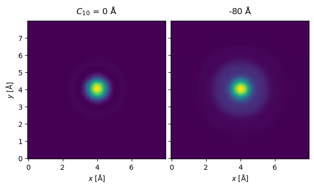
To include defocus, spherical aberration and other phase aberrations, we should define a contrast transfer function. Here we create one with a spherical aberration of \(8 \ \mu m\), the defocus is adjusted to the according Scherzer defocus.

Cs = 8e-6 * 1e10  # 8 micrometers

ctf = abtem.CTF(Cs=0, defocus=[0, 80], energy=s_matrix.energy)

We always ensure that the interpolation factor is sufficiently small to avoid self-interaction errors. We can check that by showing the equivalent probe at the entrance and exit plane.

s_matrix.dummy_probes(ctf=ctf).show(explode=True);

We should also check that our real space sampling is good enough for detecting electrons at our desired detector angles. In this case up to \(\sim 200 \ \mathrm{mrad}\). See our description of sampling.

s_matrix.cutoff_angles

(196.99522495070337, 196.99522495070337)

Create a detector and a scan

detectors = abtem.FlexibleAnnularDetector()

flexible_measurement = s_matrix.scan(
    detectors=detectors, ctf=ctf, reduction_scheme="multiple-rechunk"
)

Depending on the amount of memory available it can be necessary to limit the number of workers.

flexible_measurement.compute(num_workers=8);

<abtem.measurements.PolarMeasurements at 0x1c9113890>

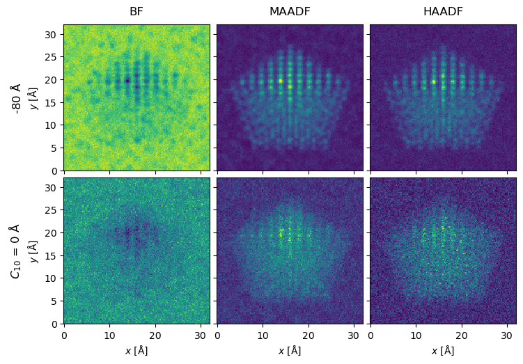
Integrate measurements

The measurements are integrated to obtain the bright field, medium-angle annular dark field and high-angle annular dark field signals.

bf_measurement = flexible_measurement.integrate_radial(0, s_matrix.semiangle_cutoff)
maadf_measurement = flexible_measurement.integrate_radial(45, 150)
haadf_measurement = flexible_measurement.integrate_radial(70, 190)

measurements = abtem.stack(
    [bf_measurement, maadf_measurement, haadf_measurement], ("BF", "MAADF", "HAADF")
)

Postprocessing

filtered_measurements = measurements.gaussian_filter(0.20).interpolate(0.2)

filtered_measurements.show(
    explode=True,
    figsize=(14, 5),
);

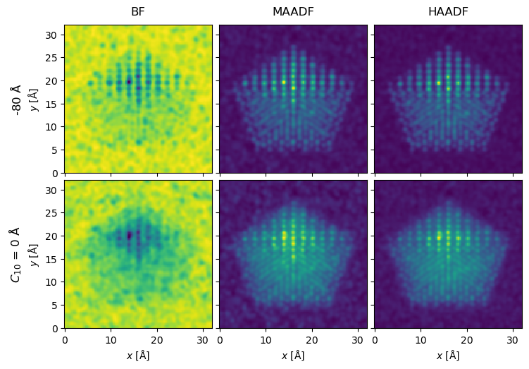
noisy_measurements = filtered_measurements.poisson_noise(dose_per_area=2e4)

noisy_measurements.show(
    explode=True,
    figsize=(14, 5),
    # cbar=True,
);