Show code cell source

Hide code cell source

import matplotlib.pyplot as plt
from ase.build import graphene
from ase.io import write

import abtem

STEM quickstart

This notebook demonstrates a basic simulation of a scanning transmission electron microscopy image of graphene with a silicon dopant.

Configuration

We start by (optionally) setting our configuration. See documentation for details.

abtem.config.set(
    {
        "device": "cpu",
        "fft": "fftw",
        "diagnostics.task_progress": True,
        "diagnostics.progress_bar": "tqdm",
    }
);

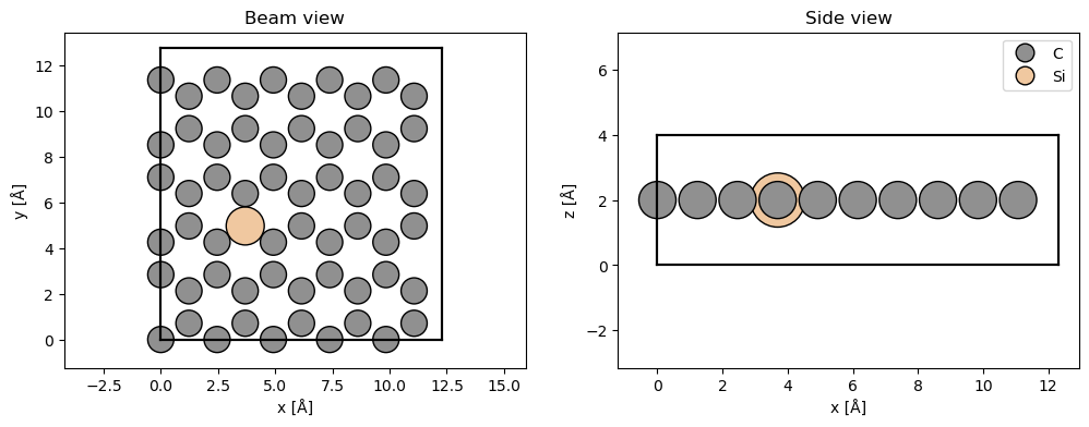
Atomic model

We create an orthogonal graphene cell. See our walkthough or our tutorial on atomic models.

atoms = abtem.orthogonalize_cell(graphene(vacuum=2))

atoms = atoms * (5, 3, 1)

We dope the graphene with silicon by changing the atomic number of one of the atoms.

atoms.numbers[17] = 14

fig, (ax1, ax2) = plt.subplots(1, 2, figsize=(12, 4))
abtem.show_atoms(atoms, ax=ax1, title="Beam view", numbering=False, merge=False)
abtem.show_atoms(atoms, ax=ax2, plane="xz", title="Side view", legend=True);

Potential

We create an ensemble of potentials using the frozen phonon model. See our walkthrough on frozen phonons.

frozen_phonons = abtem.FrozenPhonons(atoms, 8, sigmas=0.1)

We create a potential from the frozen phonons model, see walkthrough on potentials.

potential = abtem.Potential(frozen_phonons, sampling=0.05)

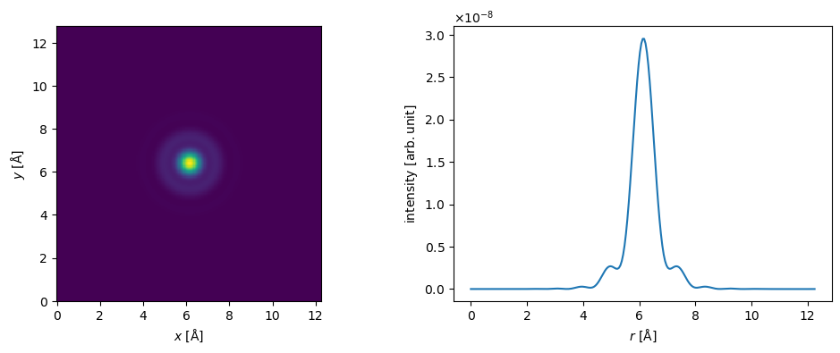
Wave function

We create a probe wave function at an energy of \(80 \ \mathrm{keV}\), an objective aperture of \(30 \ \mathrm{mrad}\), a spherical aberration of \(10 \ \mu\mathrm{m}\) and Scherzer defocus. See our walkthrough on wave functions.

Partial temporal coherence is neglected here, see our tutorial on partial coherence.

probe = abtem.Probe(energy=80e3, semiangle_cutoff=25, Cs=10e4, defocus="scherzer")
probe.grid.match(potential)

print(f"defocus = {probe.aberrations.defocus} Å")
print(f"FWHM = {probe.profiles().width().compute()} Å")

defocus = 79.14274499114904 Å
FWHM = 0.8963562846183777 Å

We show the profile of the probe.

fig, (ax1, ax2) = plt.subplots(1, 2, figsize=(12, 4))
probe.show(ax=ax1)
probe.profiles().show(ax=ax2);

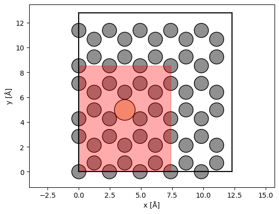
Scan

We select a scan region using fractional coordinates. We scan at the Nyquist frequency, allowing us to interpolate the measurements below.

grid_scan = abtem.GridScan(
    start=(0, 0),
    end=(3 / 5, 2 / 3),
    sampling=probe.aperture.nyquist_sampling,
    fractional=True,
    potential=potential,
)

fig, ax = abtem.show_atoms(atoms)

grid_scan.add_to_plot(ax)

Scan and detect

We use a flexible annular detector, this will let us choose the detector angles after the running multislice.

detector = abtem.FlexibleAnnularDetector()

We run the scanned multislice algorithm. See our walkthrough on scanning and detecting.

flexible_measurement = probe.scan(potential, scan=grid_scan, detectors=detector)

flexible_measurement.compute();

<abtem.measurements.PolarMeasurements at 0x1c9657b10>

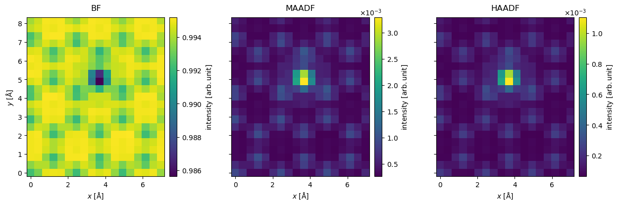
Integrate measurements

The measurements are integrated to obtain the bright field, medium-angle annular dark field and high-angle annular dark field signals.

bf_measurement = flexible_measurement.integrate_radial(0, probe.semiangle_cutoff)
maadf_measurement = flexible_measurement.integrate_radial(50, 150)
haadf_measurement = flexible_measurement.integrate_radial(90, 200)

The measurements are stacked and shown as an exploded plot.

measurements = abtem.stack(
    [bf_measurement, maadf_measurement, haadf_measurement], ("BF", "MAADF", "HAADF")
)

measurements.show(
    explode=True,
    figsize=(14, 5),
    cbar=True,
);

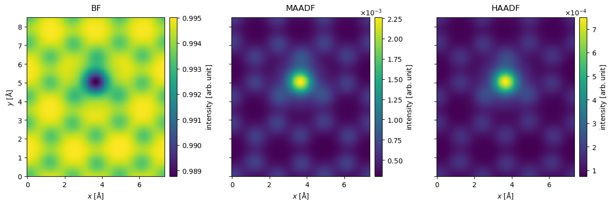
Postprocessing

Typically some post-processing steps are necessary to obtain the final results, see our walkthrough on scanning and detecting for more details

The measurements are interpolated to a sampling rate of \(0.05 \ \mathrm{Å / pixel}\).

interpolated_measurements = measurements.interpolate(0.05)

We can simulate partial spatial coherence by applying a gaussian filter. The standard deviation of the filter is \(0.3 \ \mathrm{Å}\), the approximate size of the electron source.

filtered_measurements = interpolated_measurements.gaussian_filter(0.3)

The interpolated and filtered measurements shown as an exploded plot.

filtered_measurements.show(
    explode=True,
    figsize=(14, 5),
    cbar=True,
);

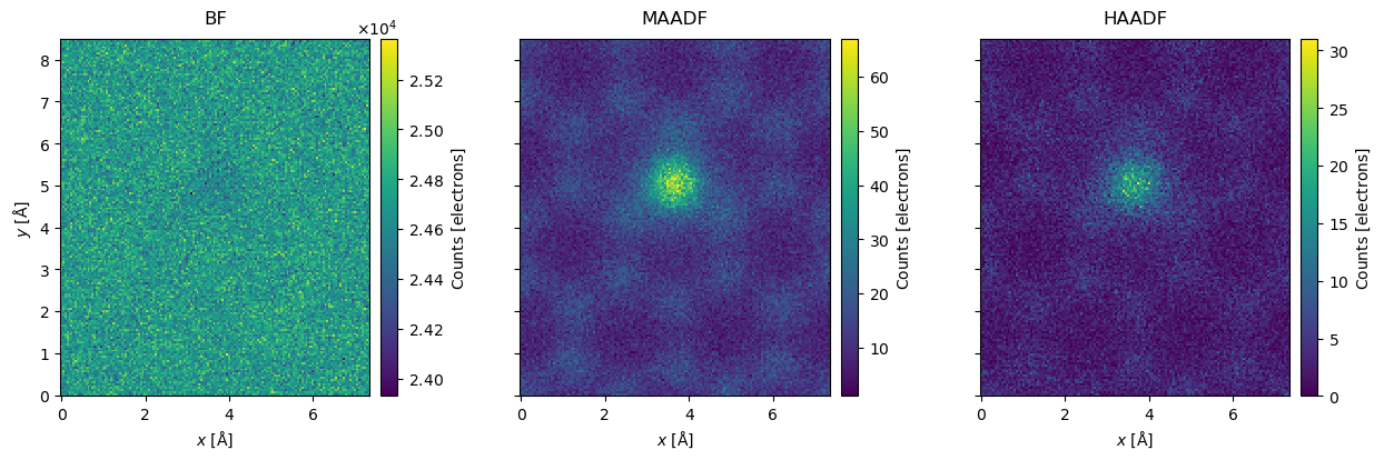
We simulate a finite electron dose of \(10^7 \ \mathrm{e}^- / \mathrm{Å}^2\) by applying poisson noise

noisy_measurements = filtered_measurements.poisson_noise(dose_per_area=1e7)

noisy_measurements.show(
    explode=True,
    figsize=(14, 5),
    cbar=True,
);

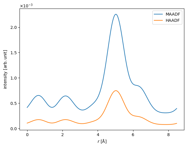
Showing the results as a line profile often provides a better sense of relative intensities.

line_profile = filtered_measurements.interpolate_line(
    start=(1 / 2, 0), end=(1 / 2, 1), fractional=True
)

line_profile[1:].show(legend=True);