Bloch-wave simulations#
Bloch-wave simulations are implemented in abTEM as an alternative to the multislice simulations, offering advantages under certain conditions. Bloch waves allow for simulations of structures with arbitrary crystal rotations and arbitrary unit cells, which are difficult to handle in multislice due to the requirement of orthogonal and periodic unit cells. Bloch waves are efficient for crystals described by small unit cells, but the computational cost in time and memory grows approximately linearly with the volume the unit cell. Hence, they become prohibitively expensive for large unit cells.
In this tutorial, we go through how to perform Bloch-wave simulations as implemented in abTEM, and compare the simulation results to multislice.
Atomic model#
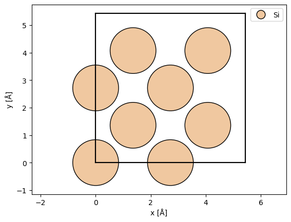
We define an atomic structure using ASE. If you are used to simulating multislice, the main difference is that we should only define a single unit cell. The computational cost in time and memory grows approximately linearly with the volume the unit cell. Here, we a conventional unit cell of silicon.
atoms = ase.build.bulk("Si", cubic=True)

abtem.show_atoms(atoms, legend=True);
The structure factor#
The structure factor is calculated using the independent atom model, as a superposition of atomic scattering factors:
\( F(\mathbf{g}) = \sum_{j} f_j(g) \exp(-2\pi i \mathbf{g} \cdot \mathbf{r}_j) \)
where \(f_j(g)\) is the atomic scattering factor of the \(j\)’th atom. The Bloch-wave code uses the same parametrizations of the scattering factors as multislice, see our description in our walkthrough on potentials.
Here, we create a StructureFactor object representing the structure factor. We provide the two required keyword arguments: atoms we created above, and the maximum spatial frequency g_max given in \(\mathrm{Å}^{-1}\) defines the maximum spatial frequency of the structure factor. Increasing g_max is equivalent to making the sampling (pixel size) smaller in a multislice simulation. As we describe later on, the \(k\)-vector of the simulated diffraction patterns, is half that of the structure factor.
When set to “auto” abTEM will attempt to determine the lattice centering, but default to primitive, when that fails.
g_max = 12.0

structure_factor = abtem.StructureFactor(
    atoms, g_max=g_max, parametrization="lobato", centering="F"
)
As other object in abTEM, we can build the StructureFactor to get an array representation.
structure_factor_array = structure_factor.build().compute()
The structure factor is represented as a 1D array with an item for each reciprocal space vector. The reciprocal space vectors may be retrieved as a sequence of Miller indices (.hkl) or as reciprocal vectors (.g_vec) in units of \(1/\mathrm{Å}\).
print(structure_factor_array.array.shape)
(289437,)
A dictionary mapping from a tuple of miller indices, (\(hkl\)), to the complex structure factor \(F_{hkl}\) can be obtained using the .to_dict method.
structure_factor_dict = structure_factor_array.to_dict()

structure_factor_dict[(0, 0, 0)]
np.complex128(0.2916122618483982+0j)
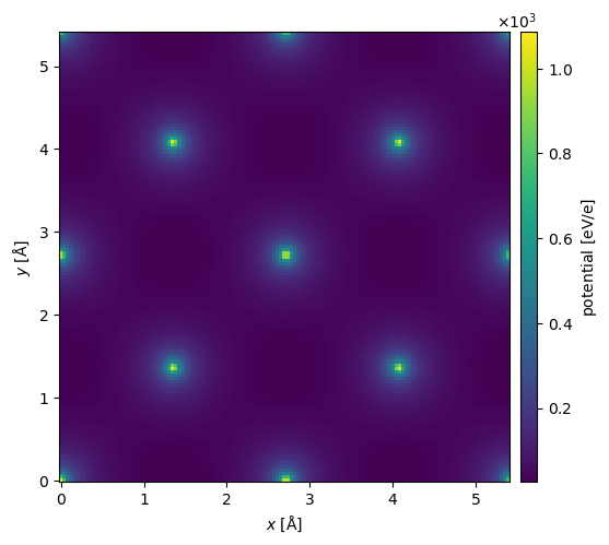
We can get the potential from the structure factor using a 3D Fourier transform
\( V(\mathbf{r}) = \frac{4 \pi \epsilon_0}{2 \pi a_0 e} \int F(g) \exp(2\pi i \mathbf{g}\cdot \mathbf{r}) \mathrm{d}\mathbf{r} \quad , \)
where \(\epsilon_0\) is the vaccum permitivity, \(a_0\) is the Bohr radius and \(e\) is the electron charge. Note that we use the unit convention from ASE, as described here.
You can get the full 3D potential as a NumPy array using the .get_potential_3d method. The projected potential as PotentialArray object, which may be used in a normal abTEM multislice simulation, can be obtained using get_projected_potential. This is currently only implemented for orthogonal unit cells.
potential = structure_factor.get_projected_potential(slice_thickness=0.1)
potential.show(cbar=True);
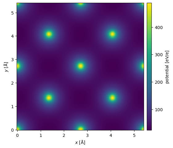
We can approximate the inclusion of phonons by providing a thermal_sigma, which will apply a Debye-Waller factor to the structure factor, effectively, blurring the potential in real space
\( F(\mathbf{g}) = \sum_{j} f_j(g) \exp(-2\pi i \mathbf{g} \cdot \mathbf{r}_j) \exp(-2 \pi^2 \sigma^2 g) . \)
In, addition we can add an imaginary component to emulate absorption, with a typical but not generally very well justified value of 10%:
\( F_{absorption}(g) = F(g) + 0.1 i F(g). \)
structure_factor_thermal = abtem.StructureFactor(
    atoms,
    g_max=g_max,
    parametrization="lobato",
    centering="F",
    thermal_sigma=0.078,
)
potential_phonons = structure_factor_thermal.get_projected_potential(slice_thickness=0.1)

potential_phonons.show(cbar=True);
Crystallographic literature typically tabulates thermal vibrations as the Debye–Waller B-factor, related to the displacement standard deviation by \(B = 8\pi^2\sigma^2\). Since version 1.0.10, the helper functions abtem.atoms.sigma_to_B and abtem.atoms.B_to_sigma convert between the two conventions.
The displacements may also be anisotropic: thermal_sigma accepts a 3-tuple \((\sigma_x, \sigma_y, \sigma_z)\) applied to all atoms, a dict mapping element symbols to 3-tuples, or an \((N, 3)\) array of per-atom values.
from abtem.atoms import B_to_sigma, sigma_to_B

B = sigma_to_B(0.078)
print(f"σ = 0.078 Å corresponds to B = {B:.3f} Ų")

structure_factor_aniso = abtem.StructureFactor(
    atoms,
    g_max=g_max,
    parametrization="lobato",
    centering="F",
    thermal_sigma=(0.078, 0.078, 0.11),
)
σ = 0.078 Å corresponds to B = 0.480 Ų
Bloch waves#
We then go on to calculate the dynamical diffraction.
A Bloch wave is included in the simulation if, for a given incident direction, it is close enough to the Bragg condition. The deviation of the reflection from exact Bragg condition is measured by the excitation error \(s_g\). abTEM always assumes propagation from negative to postive \(z\); thus for a given implied rotation of the reciprocal lattice vectors, the excitation error is calculated as \( s_g = -g_z - \frac{g^2}{2 k_0} \ , \) where the Ewald sphere is approximated as a parabola.
For a given orientation, the \(i\)’th Bloch waves is included if \( |s_{g,i}| \leq s_{g,max} \ . \)
You can control the maximum excitation error using the sg_max keyword.
We may also select a \(g_{max}\), which cannot exceed half that of the structure factor, in order to include all possible couplings between the Bloch waves.
sg_max = 0.2

bloch_waves = abtem.BlochWaves(
    structure_factor=structure_factor, energy=200e3, sg_max=sg_max, centering="F"
)

print(structure_factor.g_max, bloch_waves.g_max)
12.0 6.0
Once we have defined a structure factor, an energy and decided how many Bloch waves to include, our simulation is defined.
The dropdown goes through how abTEM calculates the structure matrix and the final simluation output.
The first step is calculating the structure matrix, \(\mathbf{A}\), this is a square matrix with the same number of rows as the number of excited beams considered in the simulation. We define the diagonal elements as
\( A_{ii} = \frac{2 k_0 s_g}{\sqrt{1 + g_{z,i} / k_0}} \)
and the off-diagonal elements as
\( A_{ij} = \frac{U_{g_i - g_j}}{\sqrt{1 + g_{z,i} / k_0} \sqrt{1 + g_{z,j} / k_0}}, \)
where
\( U_{g} = F_g. \)
The scattering matrix is given as
\( \mathbf{S} = \mathbf{M} \exp\left(\frac{2\pi i t}{2 k_0} \mathbf{A}\right) \mathbf{M}^{-1} \)
where \(\mathbf{M}\) is a diagonal matrix with
\( M_{ii} = \frac{1}{\sqrt{1+ g_z / k_0}} \ . \)
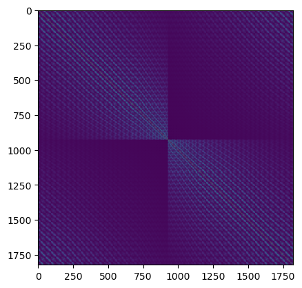
We can get the structure matrix as follows.
structure_matrix = bloch_waves.calculate_structure_matrix()
plt.figure()
plt.imshow(np.log(np.abs(1 + 1e3 * structure_matrix.compute())));
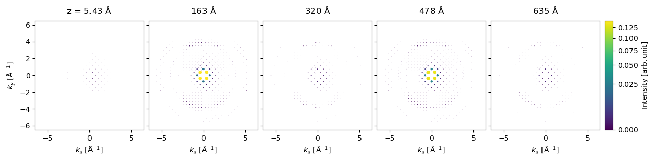
We can run our Bloch-wave simulation using the calculate_diffraction_patterns method, which takes the keyword thicknesses which can be a single thickness or a sequence of thicknesses. Here, we will get the results for each thickness of \(5.43 \ \mathrm{Å}\) up to \(645 \ \mathrm{Å}\).
If you come from a multislice background, one major difference is that large thicknesses are not more expensive than small thicknesses in a Bloch-wave simulation. (When the typical eigendecomposition is used for calculating the scattering.)
bloch_waves.hkl
array([[ 0,  0,  0],
       [ 0,  2,  0],
       [ 0,  4,  0],
       ...,
       [-1, -3, -1],
       [-1, -1,  1],
       [-1, -1, -1]], shape=(1821, 3))
thicknesses = np.arange(5.43, 645, 5.43)

diffraction_thickness_series = bloch_waves.calculate_diffraction_patterns(thicknesses)

diffraction_thickness_series.compute();
diffraction_thickness_series.shape
(118, 1821)
The output can be plotted for every 29th thickness (ie. every \(158 \ \mathrm{Å}\)).
diffraction_thickness_series[::29].block_direct().show(
    explode=True,
    scale=.2,
    power=0.5,
    annotations=False,
    figsize=(14, 5),
    common_color_scale=True,
    cbar=True,
);
Exporting results#
You can export the results to NumPy array by simply getting the array and the matching miller indices
diffraction_thickness_series.array
diffraction_thickness_series.miller_indices
array([[ 0,  0,  0],
       [ 0,  2,  0],
       [ 0,  4,  0],
       ...,
       [-1, -3, -1],
       [-1, -1,  1],
       [-1, -1, -1]], shape=(1821, 3))
abTEM supports conversion to several other formats, a good choice here might be an Xarray DataArray.
Note: You need to install Xarray to use this.
data_array = diffraction_thickness_series.to_data_array()
data_array
<xarray.DataArray (z: 118, hkl: 1821)> Size: 2MB
array([[9.97397596e-01, 6.73824151e-33, 1.14500432e-04, ...,
        3.55769272e-08, 3.03498799e-08, 2.66860012e-09],
       [9.90381509e-01, 2.81009909e-32, 4.68946651e-04, ...,
        1.60062728e-07, 1.00521348e-07, 1.21364880e-08],
       [9.79390603e-01, 6.25885172e-32, 1.07472171e-03, ...,
        3.86241899e-07, 2.01785047e-07, 2.93774299e-08],
       ...,
       [9.82080387e-01, 1.79856801e-28, 1.86839195e-03, ...,
        2.27828672e-06, 3.67562955e-05, 4.16252281e-07],
       [9.88746689e-01, 1.72619477e-28, 1.51024794e-03, ...,
        1.73225913e-06, 3.78267688e-05, 5.30004765e-07],
       [9.91603373e-01, 1.65068710e-28, 1.15464472e-03, ...,
        1.20719822e-06, 3.93324802e-05, 6.82705065e-07]],
      shape=(118, 1821))
Coordinates:
  * z        (z) float64 944B 5.43 10.86 16.29 21.72 ... 624.4 629.9 635.3 640.7
  * hkl      (hkl) <U10 73kB '0 0 0' '0 2 0' '0 4 0' ... '-1 -1 1' '-1 -1 -1'
    k        (hkl) float64 15kB 0.0 0.3683 0.7366 1.105 ... 0.6108 0.319 0.319
Attributes:
    long_name:  intensity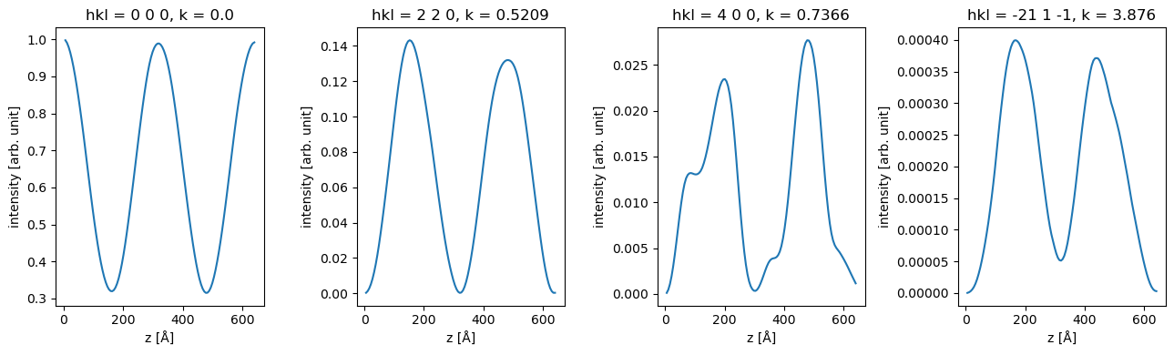
units: arb. unitWe can use xarray to slice the data, for example to show the intensity of of specific.
fig, axes = plt.subplots(1, 4, figsize=(13, 4))

for ax, hkl in zip(axes, ["0 0 0", "2 2 0", "4 0 0", "-21 1 -1"]):
    data_array.sel(hkl=hkl).plot(hue="hkl", ax=ax)

plt.tight_layout()
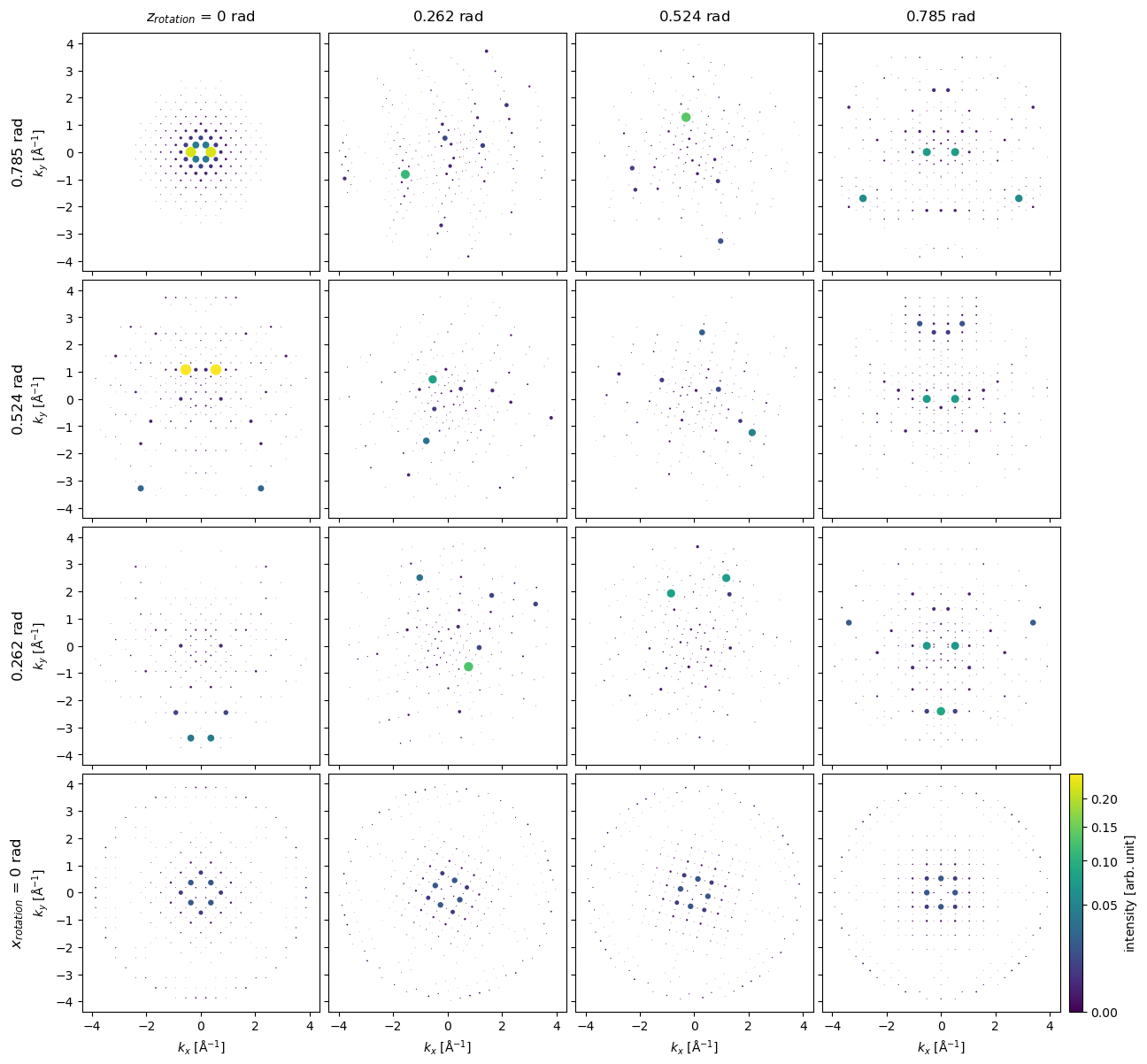
Rotations#
We can get diffraction intensities from other directions using the rotations method. Here, we rotate about \(z\) at \(4\) different angles between \(0\) and \(45 \ \mathrm{deg}\), for each \(z\) rotation we also rotate around \(x\) at \(5\) different angles between \(0\) and \(45 \ \mathrm{deg}\), i.e. resulting in \(16\) different simulations.
bloch_waves = abtem.BlochWaves(
    structure_factor=structure_factor, energy=200e3, sg_max=sg_max, centering="F"
)

x = np.linspace(0, np.pi / 4, 4)
z = np.linspace(0, np.pi / 4, 4)

ensemble = bloch_waves.rotate("z", z, "x", x)
The previous operation produces a BlochwaveEnsemble object, we run the same calculate_diffraction_patterns method to create the tasks for running a Bloch-wave simulation for each direction.
Note: this may take up to 15 min to complete.
diffraction_patterns = ensemble.calculate_diffraction_patterns(thicknesses=1000)

diffraction_patterns.array
|
||||||||||||||||
diffraction_patterns.compute()
<abtem.measurements.IndexedDiffractionPatterns at 0x1d252f4d0>
diffraction_patterns.shape
(4, 4, 11843)
diffraction_patterns = diffraction_patterns.remove_low_intensity(1e-6)
diffraction_patterns.crop(k_max=4).block_direct().show(
    explode=True,
    scale=0.2,
    power=0.5,
    annotation_kwargs={"threshold": 1},
    figsize=(14, 14),
    cbar=True,
    common_color_scale=True
);
Arbitrary rotations may be given as a sequence of Euler angles, for example, to rotate about a vector pointing along \((-1, 1, 0)\), we can rotate by \(\pi/4\) around \(z\), apply the desired rotations around \(x\), and then rotate back by \(-\pi/4\) around \(z\).
z = np.tile([np.pi / 4], (4,))
x = np.linspace(0, np.pi / 2, 4)

rotations = np.array([z, x, -z]).T
ensemble = bloch_waves.rotate("zxz", rotations)

diffraction_patterns = ensemble.calculate_diffraction_patterns(1000).compute()
diffraction_patterns.crop(k_max=4).block_direct().show(
    explode=True,
    scale=0.2,
    power=0.5,
    annotation_kwargs={"threshold": 1},
    figsize=(14, 14),
    cbar=True,
    common_color_scale=True
);

Comparison to multislice#
g_max = 12

structure_factor = abtem.StructureFactor(
    atoms, g_max=g_max, parametrization="lobato", centering="F", thermal_sigma=0.078
)
potential_sf = structure_factor.get_projected_potential(slice_thickness=0.5)

potential_sf.sampling
(0.04082706766917293, 0.04082706766917293)
parametrization = abtem.parametrizations.LobatoParametrization(
    sigmas={"Si": 0.078}
)

potential = (
    abtem.Potential(
        atoms,
        sampling=potential_sf.sampling,
        slice_thickness=0.1,
        projection="finite",
        parametrization=parametrization,
    )
    .build()
    .compute(progress_bar=False)
)
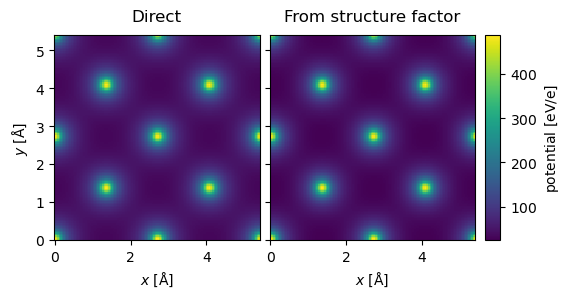
stack = abtem.stack(
    (potential.project(), potential_sf.project()), ("Direct", "From structure factor")
).compute()

stack.show(explode=True, common_color_scale=True, cbar=True);
pw = abtem.PlaneWave(energy=200e3)
nz = int(1086 / potential.thickness)
repeated_potential = abtem.CrystalPotential(
potential, repetitions=[1, 1, nz], exit_planes=potential.num_slices
)
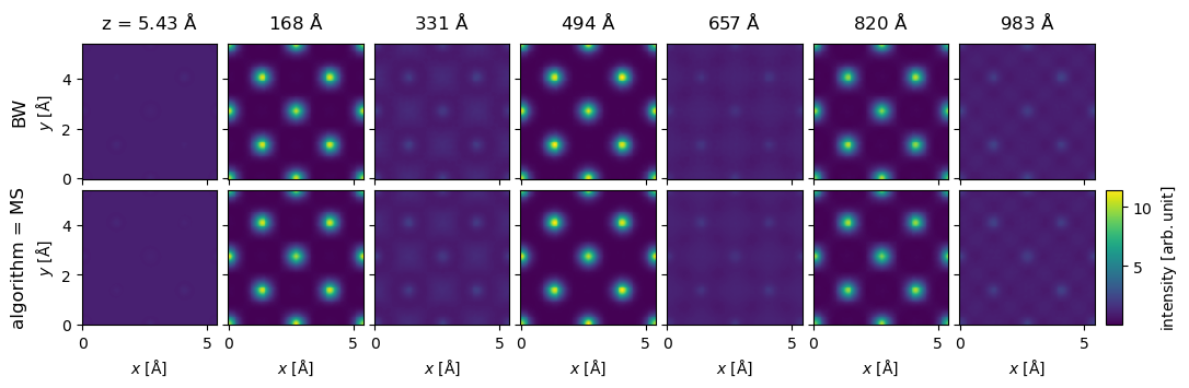
exit_waves_ms = pw.multislice(potential=repeated_potential).compute()
bloch_waves = abtem.BlochWaves(
    structure_factor=structure_factor, energy=200e3, sg_max=sg_max
)

len(bloch_waves)
1821
exit_waves_bw = bloch_waves.calculate_exit_waves(
    repeated_potential.exit_thicknesses, gpts=exit_waves_ms.gpts
)
/Users/tomasusi/git/abTEM/abtem/bloch/dynamical.py:1659: PerformanceWarning: Increasing number of chunks by factor of 27
  array = da.blockwise(
exit_waves_bw.shape
(201, 133, 133)
exit_waves_ms.shape
(201, 133, 133)
stack = abtem.stack(
    [exit_waves_bw, exit_waves_ms],
    axis_metadata={"label": "algorithm", "values": ["MS", "BW"]},
    axis=1,
).compute();
stack[1::30].show(explode=True, figsize=(12, 4), cbar=True, common_color_scale=True);
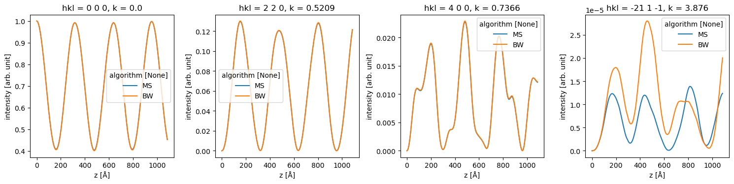
stacked_diffraction = (
    stack.diffraction_patterns().index_diffraction_spots(cell=atoms)
)
The difference below for the very weak [-21 1 -1] spot is mostly due to a slightly unconverged Bloch-wave calculation.
data_array = stacked_diffraction.to_data_array()

fig, axes = plt.subplots(1, 4, figsize=(15, 4))

for ax, hkl in zip(axes, ["0 0 0", "2 2 0", "4 0 0", "-21 1 -1"]):
    data_array.sel(hkl=hkl).plot(hue="algorithm", ax=ax)

plt.tight_layout()