import abtem
import ase
import matplotlib.pyplot as plt
import numpy as np
import pandas as pd
from abtem.bloch import BlochWaves, StructureFactor

# nicer formatting for online display of pandas dataframes
pd.set_option("display.float_format", "{:.3f}".format)
pd.set_option("display.max_columns", 15)
pd.set_option("display.max_rows", 8)

Bloch wave quickstart

This is a short example of running an electron diffraction simulation of zirconium oxide. See our tutorial for a more in depth description of abTEM’s implementation of Bloch waves.

Configuration

We start by (optionally) setting our configuration. See documentation for details.

abtem.config.set(
    {
        "precision": "float64",
        "device": "cpu",
    }
);

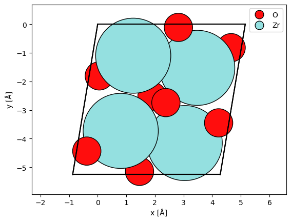
Atomic model

We import an atomic model of zirconium oxide from the materials project.

As opposed to multislice simulations, we should not repeat the atoms. Note also that simulating a non-orthogonal unit cell is not an issue with Bloch waves.

atoms = ase.io.read("data/ZrO2.cif")

We rotate the atoms by \(90 \ \mathrm{deg}\) around \(x\).

atoms.rotate("x", 90, rotate_cell=True)

abtem.show_atoms(atoms, legend=True, plane="xy")

(<Figure size 640x480 with 1 Axes>, <Axes: xlabel='x [Å]', ylabel='y [Å]'>)

Structure factor

We create the StructureFactor, we should provide at least the atoms and the magnitude, g_max, of the maximum included reciprocal lattice vector. In addition we can select a parametrization and apply a Debye-Waller factor by setting thermal_sigma.

structure_factor = StructureFactor(
    atoms,
    g_max=6.0,
    parametrization="lobato",
    thermal_sigma=0.0,
)

Bloch waves

We define the BlochWaves by providing the structure factor, an electron energy and the excitation error(sg_max). The included Bloch waves is those with a magnitude less than half g_max and with an excitation error (approximate distance to the Ewald) of less than sg_max.

sg_max = 0.12

bloch_waves = BlochWaves(structure_factor=structure_factor, energy=200e3, sg_max=sg_max)

print(structure_factor.g_max, bloch_waves.g_max)

6.0 3.0

The cost of Bloch wave simulation scales as cubed with the number of Bloch waves, hence we check the number here. For smaller systems \(8000\) or more Bloch waves may be time-consuming.

print(len(bloch_waves))

1043

We also print the size of the structure matrix.

print(bloch_waves.structure_matrix_nbytes * 1e-9, "GB")

0.017405584 GB

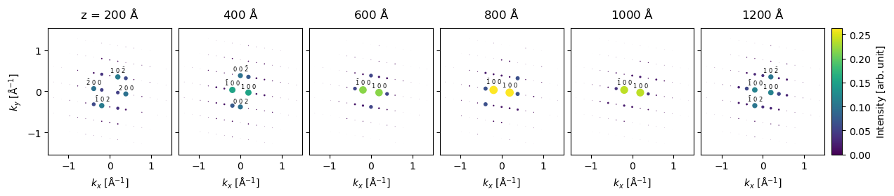
We set up a simulation choosing a range of thicknesses in \(\mathrm{Å}\).

thicknesses = np.arange(0, 1210, 10)

diffraction = bloch_waves.calculate_diffraction_patterns(thicknesses=thicknesses)

diffraction.compute()

<abtem.measurements.IndexedDiffractionPatterns at 0x1be364ad0>

We show every \(20\)’th the results cropped to a maximum scattering vector of \(k_{max}=1.5 \ \mathrm{Å}\).

diffraction[20::20].block_direct().crop(k_max=1.5).show(
    explode=True,
    scale=0.1,
    figsize=(14, 5),
    annotation_kwargs={"threshold": 0.08, "fontsize": 6},
    cbar=True,
    common_color_scale=True,
);

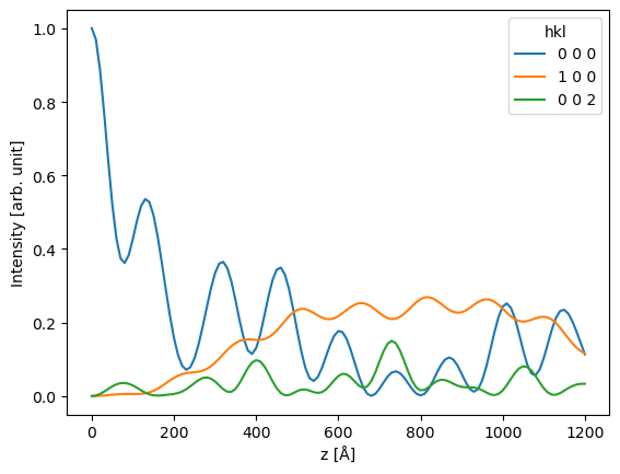
To perform a more quantitative analysis, we can get the data as pandas dataframe.

df = diffraction.remove_low_intensity(0.05).to_dataframe()
df

hkl	0 0 0	0 0 2	0 0 -2	1 0 0	1 0 -2	2 0 0	2 0 -2	-2 0 0	-2 0 2	-1 0 0	-1 0 2
z [Å]
0	1.000	0.000	0.000	0.000	0.000	0.000	0.000	0.000	0.000	0.000	0.000
10	0.969	0.001	0.001	0.000	0.000	0.001	0.001	0.001	0.001	0.000	0.000
20	0.887	0.006	0.006	0.001	0.001	0.004	0.003	0.004	0.003	0.001	0.001
30	0.770	0.012	0.012	0.002	0.003	0.009	0.007	0.009	0.007	0.002	0.003
...	...	...	...	...	...	...	...	...	...	...	...
1170	0.202	0.028	0.028	0.143	0.049	0.006	0.043	0.006	0.043	0.143	0.049
1180	0.175	0.031	0.031	0.131	0.063	0.015	0.033	0.015	0.033	0.131	0.063
1190	0.144	0.033	0.033	0.122	0.082	0.033	0.023	0.033	0.023	0.122	0.082
1200	0.114	0.034	0.034	0.116	0.102	0.057	0.017	0.057	0.017	0.116	0.102

121 rows × 11 columns

ax = df[["0 0 0", "1 0 0", "0 0 2"]].plot()
ax.set_ylabel("Intensity [arb. unit]");

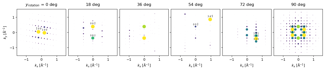
Single axis rotation

To simulate a rotated sample we use the rotate method obtaining a BlochWavesEnsemble.

rotations = np.linspace(0, 90, 6)

rotated_bloch_waves = bloch_waves.rotate("y", rotations, degrees=True)

rotated_bloch_waves.shape

(6,)

We setup the simulation for a single thickness.

rotated_diffraction = rotated_bloch_waves.calculate_diffraction_patterns(
    thicknesses=500.0
)

And run the simulation.

rotated_diffraction.compute(num_workers=3);

Finally showing the result.

rotated_diffraction.block_direct().crop(k_max=1.5).show(
    explode=True,
    scale=0.12,
    figsize=(14, 5),
    annotation_kwargs={"threshold": 0.05, "fontsize": 6},
);

Precession electron diffraction

In this example, we will calculate a precession electron diffraction pattern. We choose a precession angle of \(50 \ \mathrm{mrad}\) and \(100\) steps.

precession_angle = 50 * 1e-3

azimuthal_angles = np.linspace(0, 2 * np.pi, num=100, endpoint=False)

tilt = precession_angle * np.stack(
    [np.cos(azimuthal_angles), np.sin(azimuthal_angles)], axis=1
)

tilt.shape

(100, 2)

The sample is rotated around \(x\) then \(y\) as given by each row of the tilt array. For more general and multidimensional rotations refer to tutorial.

precessed_bloch_waves = bloch_waves.rotate("xy", tilt, degrees=False)

precessed_diffraction = precessed_bloch_waves.calculate_diffraction_patterns(
    thicknesses=300.0
)

abTEM parallelizes over rotations, however, due to the large memory requirement of Bloch wave simulations the number of workers should be limited.

precessed_diffraction.compute(num_workers=4);

<abtem.measurements.IndexedDiffractionPatterns at 0x1d9039350>

We integrate over the precession angles using the mean method.

integrated = precessed_diffraction.mean(0)

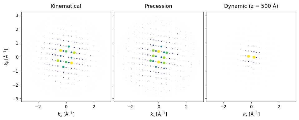
kinematical = bloch_waves.get_kinematical_diffraction_pattern()

stack = (
    abtem.stack(
        (kinematical, integrated, diffraction[50]),
        ("Kinematical", "Precession", "Dynamic (z = 500 Å)"),
    )
    .block_direct()
    .show(annotations=False, scale=0.1, explode=True, figsize=(10, 4))
)

# this cell produces a thumbnail for the online documentation

visualization = integrated.block_direct().crop(80).show(annotations=False, scale=0.12)
visualization.axis_off()
plt.savefig(
    "../thumbnails/blochwave_quickstart.png", bbox_inches="tight", pad_inches=0
)