import abtem
import ase
import matplotlib.pyplot as plt
import numpy as np
from abtem.finite_difference import DivergedError
from abtem.multislice import FourierMultislice, RealSpaceMultislice

abtem.config.set({"device": "cpu"});
abtem.config.set({"diagnostics.progress_bar": False});

Real-space multislice

For certain kinds of situations, it is necessary to run the multislice algorithm fully in real space and not rely on Fourier transforms. This will incur a performance penalty, however, so this method is not used by default.

After the initial simple implementation by Jacob Madsen, this functionality was improved and expanded by Mathijs van den Doel and Georgios Varnavides. The implementation is based on the work of Ming & Chen [MC13], and Chen et al. [CHM+25].

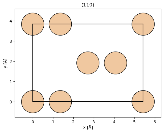
Let’s demonstrate this for Si in the (110) orientation.

desired_rotation = 45
silicon = ase.build.bulk("Si", cubic=False)

# Rotates silicon structure by 45 degrees.
rotated_silicon = silicon.copy()

rotated_silicon.rotate(desired_rotation, "x", rotate_cell=True)
rotated_silicon, transform = abtem.orthogonalize_cell(
    rotated_silicon, max_repetitions=10, return_transform=True
)

rotated_silicon.center(axis=2)

abtem.show_atoms(
    rotated_silicon, show_periodic=True, scale=0.5, title="(110)", plane="xy"
);

Create a potential. The real-space method requires slightly smaller slices for convergence.

potential_unit = abtem.Potential(
    rotated_silicon,
    slice_thickness=0.5,
    sampling=0.05,
    projection="finite",
)
potential = abtem.CrystalPotential(potential_unit, repetitions=(1, 1, 10))
plane_wave = abtem.PlaneWave(energy=200e3)
plane_wave.grid.match(potential)

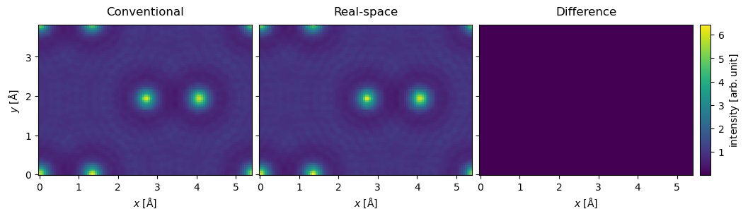
The multislice algorithm is selected by passing an algorithm object to multislice: FourierMultislice (the default) or RealSpaceMultislice, both imported from abtem.multislice. For the real-space algorithm, you can set the order of the accuracy of the finite difference derivative stencil using the derivative_accuracy keyword. The total number of terms in the series expansion is determined by a convergence criteria.

exit_wave_cms = plane_wave.multislice(
    potential,
    algorithm=FourierMultislice(), # default, can omit
)
exit_wave_rms = plane_wave.multislice(
    potential,
    algorithm=RealSpaceMultislice(),
)

abtem.stack((exit_wave_cms, exit_wave_rms, exit_wave_cms-exit_wave_rms), ("Conventional", "Real-space", "Difference")).show(
    explode=True, figsize=(12, 4), common_color_scale=True, cbar=True
);

OMP: Info #276: omp_set_nested routine deprecated, please use omp_set_max_active_levels instead.

The calculation may diverge if the slices are too thick, you can catch the DivergedError exception. A better sampling also requires a smaller slice thickness.

potential_unit = abtem.Potential(
    rotated_silicon,
    slice_thickness=2,
    sampling=0.05,
    projection="finite",
)

potential = abtem.CrystalPotential(potential_unit, repetitions=(1, 1, 10))
plane_wave = abtem.PlaneWave(energy=200e3)
plane_wave.grid.match(potential)

try:
    exit_wave_rms = plane_wave.multislice(
        potential,
        algorithm=RealSpaceMultislice(),
        lazy=False
    )
except DivergedError:
    print("Calculation diverged!")

Calculation diverged!

Advanced usage

The real-space method further allows the use of a higher-order Taylor series expansions of the multislice operator. This is particularly motivated for low energy S/TEM applications where the standard high-energy multislice approximation breaks down (below about 30 keV).

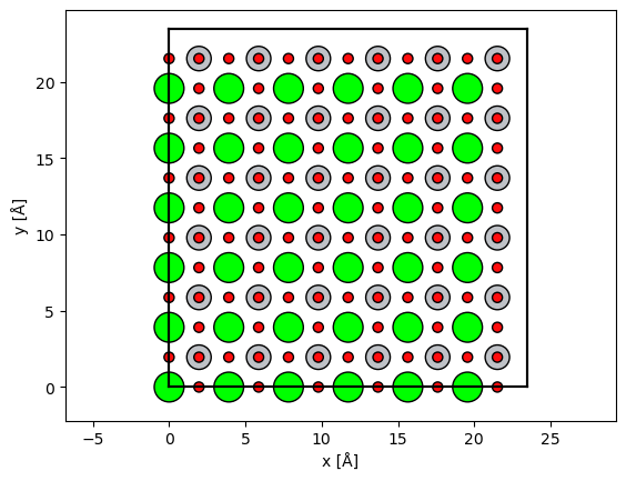
To demonstrate this, we will use STO as the specimen model.

unit_cell = ase.Atoms(
    symbols="SrTiO3",
    scaled_positions=[
        [0.0,0.0,0.0],
        [0.5,0.5,0.5],
        [0.5,0.0,0.5],
        [0.5,0.5,0.0],
        [0.0,0.5,0.5]
    ],
    cell=[3.9127,3.9127,3.9127],
    pbc=True
)

atoms = unit_cell * (6,6,24)
abtem.show_atoms(
    atoms,plane='xy',
    scale=0.5,
);

potential = abtem.Potential(
    atoms,
    gpts = (6*40,6*40),
    slice_thickness=0.5, # this needs to be small-enough to ensure real-space MS converges
    # device='gpu',
    projection='finite',
);

Focused probe

Below we showcase with a focused probe at 30 keV to demonstrate scanned measurements, but all methods also work with planewaves.

energy = 30e3
semiangle_cutoff = 20

converged_probe = abtem.Probe(
    semiangle_cutoff=semiangle_cutoff,
    energy=energy,
    # device='gpu',
).match_grid(
    potential
)

# tiny grid_scan for demo purposes
grid_scan = abtem.GridScan(
    start=(0,0),
    end=(unit_cell.cell[0,0],unit_cell.cell[1,1]),
    gpts=2,
);

Multislice algorithm objects

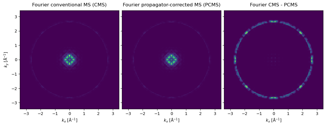
There are two new algorithm objects, where the conventional multislice operator has been renamed to FourierMultislice, with the following signatures:

@dataclass(frozen=True)
class FourierMultislice:
    order: Literal[1, 2] = 1
    expansion_scope: Literal["propagator"] = "propagator"
    conjugate: bool = False
    transpose: bool = False


@dataclass(frozen=True)
class RealSpaceMultislice:
    order: int = 1
    expansion_scope: Literal["propagator", "full"] = "propagator"
    derivative_accuracy: int = 6
    max_terms: int = 80

Conventional Fourier methods

from abtem.multislice import FourierMultislice, RealSpaceMultislice

# default is FourierMultislice(), i.e. Fourier MS of order 1
forward_exit_waves_fourier = converged_probe.multislice(
    potential=potential,
    scan = [[0,0]],
)

# FourierMultislice also supports the spherical-propagator case, i.e. order 2
forward_exit_waves_fourier_pc = converged_probe.multislice(
    potential=potential,
    scan = [[0,0]],
    algorithm=FourierMultislice(order=2)
)

# # higher-orders give a ValueError
# forward_exit_waves_fourier = converged_probe.multislice(
#     potential=potential,
#     scan = [[0,0]],
#     algorithm=FourierMultislice(order=3)
# )

# # less common parameters include conjugate and transpose options
# forward_exit_waves_fourier = converged_probe.multislice(
#     potential=potential,
#     scan = [[0,0]],
#     algorithm=FourierMultislice(conjugate=True,transpose=False)
# )

forward_exit_waves_fourier_stack = abtem.stack(
    (
        forward_exit_waves_fourier,
        forward_exit_waves_fourier_pc,
        forward_exit_waves_fourier - forward_exit_waves_fourier_pc
    ),
    (
        "Fourier conventional MS (CMS)",
        "Fourier propagator-corrected MS (PCMS)",
        "Fourier CMS - PCMS"
    )
)

forward_exit_waves_fourier_stack.diffraction_patterns().show(explode=True,figsize=(12,4));

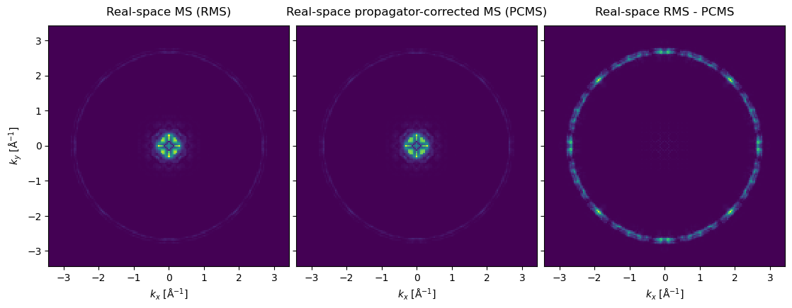
Real-space methods

# Real-space MS of order 1
# Note: we have added an antialias aperture for consistency.
forward_exit_waves_realspace = converged_probe.multislice(
    potential=potential,
    scan = [[0,0]],
    algorithm = RealSpaceMultislice()
)

# Real-space MS of order 3 in the propagator
forward_exit_waves_realspace_pc = converged_probe.multislice(
    potential=potential,
    scan = [[0,0]],
    algorithm = RealSpaceMultislice(order=3)
)

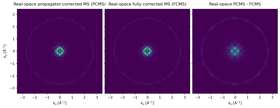
# Real-space MS of order 3 in the propagator and potential
forward_exit_waves_realspace_fc = converged_probe.multislice(
    potential=potential,
    scan = [[0,0]],
    algorithm = RealSpaceMultislice(order=3, expansion_scope="full")
)

# # Less common parameters include finite-difference derivative order and maximum exponential series terms.
# forward_exit_waves_fourier = converged_probe.multislice(
#     potential=potential,
#     scan = [[0,0]],
#     lazy=False,
#     algorithm = RealSpaceMultislice(derivative_accuracy=8,max_terms=60)
# )

forward_exit_waves_realspace_stack = abtem.stack(
    (
        forward_exit_waves_realspace,
        forward_exit_waves_realspace_pc,
        forward_exit_waves_realspace - forward_exit_waves_realspace_pc
    ),
    (
        "Real-space MS (RMS)",
        "Real-space propagator-corrected MS (PCMS)",
        "Real-space RMS - PCMS"
    )
)

forward_exit_waves_realspace_stack.diffraction_patterns().show(explode=True,figsize=(12,4));

forward_exit_waves_realspace_stack_2 = abtem.stack(
    (
        forward_exit_waves_realspace_pc,
        forward_exit_waves_realspace_fc,
        forward_exit_waves_realspace_pc - forward_exit_waves_realspace_fc
    ),
    (
        "Real-space propagator-corrected MS (PCMS)",
        "Real-space fully corrected MS (FCMS)",
        "Real-space PCMS - FCMS"
    )
)

forward_exit_waves_realspace_stack_2.diffraction_patterns().show(explode=True,figsize=(12,4));

Coherent backscattered wave

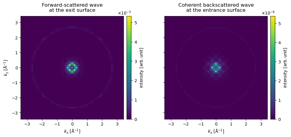
The real-space method also allows us to include the effect of backscattered electrons. Backscattering requires we keep track of the scattered waves as a function of depth, for which we use exit_planes in the potential.

Please note that this is mostly tracking the intensity lost from the forward-propagating wave – not backscattered electrons in the EBSD sense.

potential_exit_planes = abtem.Potential(
    atoms,
    gpts = (6*40,6*40),
    slice_thickness=0.5,
    exit_planes=1,
    # device='gpu',
    projection='finite',
);

forward_exit_waves_realspace_fc, backward_exit_waves_realspace_fc = converged_probe.multislice(
    potential=potential_exit_planes,
    scan = [[0,0]],
    algorithm = RealSpaceMultislice(order=3,expansion_scope="full"),
    return_backscattered = True
);

bs_exit_waves_realspace_stack = abtem.stack(
    (
        forward_exit_waves_realspace_fc[-1],
        backward_exit_waves_realspace_fc[0],
    ),
    (
        "Forward-scattered wave\nat the exit surface",
        "Coherent backscattered wave\nat the entrance surface"
    )
)

bs_exit_waves_realspace_stack.diffraction_patterns().show(explode=True,figsize=(12,4),cbar=True);

Scan and detectors

# Work with scan axes
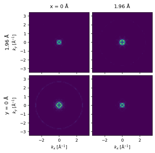
forward_exit_waves_realspace_pc_scan = converged_probe.multislice(
    potential=potential,
    scan = grid_scan,
    algorithm = RealSpaceMultislice(order=3)
)

forward_exit_waves_realspace_pc_scan.diffraction_patterns().show(explode=True);

# Work with detectors
pixelated_realspace_pc, annular_realspace_pc = converged_probe.multislice(
    potential=potential,
    scan = grid_scan,
    detectors= [abtem.PixelatedDetector(), abtem.AnnularDetector(inner=30,outer=100)],
    algorithm = RealSpaceMultislice(order=3)
).compute();

# Inclusion of backscattering simply adds an extra WavesDetector at the end
forward_pixelated_realspace_fc, forward_annular_realspace_fc, backward_exit_waves_realspace_fc = converged_probe.multislice(
    potential=potential_exit_planes,
    scan = [[0,0]],
    detectors= [abtem.PixelatedDetector(), abtem.AnnularDetector(inner=30,outer=100)],
    algorithm = RealSpaceMultislice(order=3,expansion_scope="full"),
    return_backscattered = True
).compute();