import numpy as np
from ase.build import bulk

import abtem

abtem.config.set({"diagnostics.progress_bar": False});

Ensembles

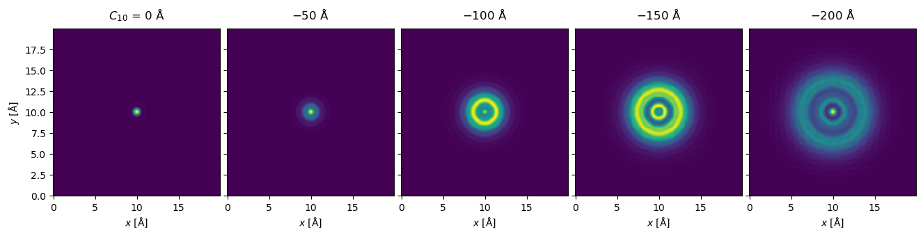
Many of the key objects in abTEM carry two kinds of axes: a set of base axes that are necessary to describe the object — for example, the \(x\) and \(y\) axes of a wave function — and any number of additional ensemble axes, which describe a collection of such objects with different parameters. A defocus series, the atomic configurations of a thermal ensemble, the positions of a probe scan, and the samples of a partially coherent source are all ensemble axes, and they are the common machinery behind most of abTEM’s “vary a parameter” workflows.

The simplest way to create an ensemble is to hand an array of values to a parameter that would normally be a single number:

probe = abtem.Probe(
    energy=100e3, extent=20, gpts=256, semiangle_cutoff=30, defocus=np.linspace(0, 200, 5)
)

waves = probe.build()

print(f"ensemble shape: {waves.ensemble_shape}, base shape: {waves.base_shape}")

waves.axes_metadata

ensemble shape: (5,), base shape: (256, 256)

type           label    coordinates
-------------  -------  ------------------------
ParameterAxis  C10 [Å]  -0.00 -50.00 ... -200.00
RealSpaceAxis  x [Å]    0.00 0.08 ... 19.92
RealSpaceAxis  y [Å]    0.00 0.08 ... 19.92

The wave functions gained a leading ParameterAxis, and its coordinates are recorded in the axes metadata (the defocus appears as the aberration coefficient \(C_{10} = -\Delta f\), following the conventions). Ensemble axes always precede the base axes in the shape of an object, and they follow the object through every operation — including into visualizations, where an ensemble axis can be browsed interactively, exploded into a grid of panels, or animated:

waves.intensity().compute().show(explode=True, figsize=(14, 4), cbar=False);

Distributions

A plain array gives every ensemble member equal importance. The abtem.distributions module creates parameter distributions that also carry weights:

• abtem.distributions.uniform — evenly spaced values with uniform weights;

• abtem.distributions.from_values — arbitrary user-defined values and weights;

• abtem.distributions.gaussian — values weighted by a (possibly multidimensional) Gaussian, as used for example to model focal spread.

For example, a Gaussian defocus distribution:

distribution = abtem.distributions.gaussian(
    center=-100, standard_deviation=50, num_samples=5, ensemble_mean=True
)

for value, weight in zip(np.array(distribution.values), distribution.weights):
    print(f"defocus: {value:7.1f} Å, weight: {weight:.3f}")

defocus:  -250.0 Å, weight: 0.010
defocus:  -175.0 Å, weight: 0.295
defocus:  -100.0 Å, weight: 0.909
defocus:   -25.0 Å, weight: 0.295
defocus:    50.0 Å, weight: 0.010

Reducing an ensemble

The ensemble_mean flag above does not change the values — it tags the axis for reduction. Whenever the ensemble is reduced — explicitly, by calling abtem.waves.reduce_ensemble, or automatically, when a detector integrates the signal during a scan — a weighted average is taken over every axis tagged with ensemble_mean=True, while untagged axes survive into the measurement so that each member can be inspected separately.

The difference is easy to see in a STEM simulation with a focal-spread distribution: with ensemble_mean=True the defocus axis is averaged away during detection, while with ensemble_mean=False it remains as an axis of the measurement:

atoms = bulk("Si", "diamond", a=5.43, cubic=True) * (2, 2, 4)
potential = abtem.Potential(atoms, sampling=0.1, slice_thickness=2)
detector = abtem.FlexibleAnnularDetector()

for ensemble_mean in (True, False):
    focal_spread = abtem.distributions.gaussian(
        center=0, standard_deviation=50, num_samples=5, ensemble_mean=ensemble_mean
    )
    probe = abtem.Probe(energy=100e3, semiangle_cutoff=30, defocus=focal_spread)

    measurement = probe.scan(potential, detectors=detector)

    print(f"ensemble_mean={ensemble_mean!s:>5}: measurement shape {measurement.shape}")

ensemble_mean= True: measurement shape (36, 36, 122, 1)
ensemble_mean=False: measurement shape (5, 36, 36, 122, 1)

(Both measurements above are lazy — the shapes are known before anything is computed.)

Multidimensional ensembles

When several parameters are given as distributions, the ensemble becomes their outer product, adding one axis per parameter:

ctf = abtem.CTF(energy=100e3, defocus=np.linspace(0, 100, 4), Cs=np.linspace(0, 1e5, 3))

print(f"ensemble shape: {ctf.ensemble_shape}")

ctf.axes_metadata

ensemble shape: (4, 3)

type           label    coordinates
-------------  -------  ------------------------
ParameterAxis  C10 [Å]  -0.00 -33.33 ... -100.00
ParameterAxis  C30 [Å]  0.00 50000.00 100000.00

A two-parameter series like this computes \(4 \times 3 = 12\) contrast transfer functions in a single, fully parallel calculation.

Parallelization over ensembles

Each member of an ensemble is independent, which allows for trivial parallelization: abTEM groups the ensemble into batches that map onto the chunks of the underlying Dask arrays, and Dask distributes them over the available resources (see the parallelization walkthrough). The batch size is controlled by the dask.chunk-size configuration option, as described in the performance tips.

The partitioning of an ensemble into Dask blocks can be inspected directly:

ctf.ensemble_blocks(2)

Array Chunk Bytes 96 B 16 B Shape (4, 3) (2, 1) Dask graph 6 chunks in 3 graph layers Data type object numpy.ndarray